1. Preface
Optical flow is a fundamental problem in computer vision that has been studied for decades. It refers to the motion of objects in an image or video sequence, which can be estimated by analyzing the spatiotemporal changes of pixel intensities. Optical flow has a wide range of applications in robotics, autonomous driving, augmented reality, and video compression, to name a few.
Despite its long history and practical importance, optical flow remains a challenging task due to various factors such as occlusion, motion blur, illumination changes, and textureless regions. Over the years, numerous algorithms and techniques have been proposed to address these issues and improve the accuracy and robustness of optical flow estimation.
In this post, we will provide an introduction to optical flow from theory to practice. We will start by introducing the basic concepts and assumptions of optical flow, followed by a survey of classic and modern optical flow methods. We will also discuss the evaluation metrics and datasets commonly used for optical flow benchmarking. Finally, we will provide some practical tips and tricks for using optical flow in real-world applications.
Whether you are a beginner in computer vision or an experienced practitioner, we hope this post will help you gain a better understanding of optical flow and its potential in various fields.
2. Coherence
How do humans predict the movement of objects? Like many other areas of computer vision, optical flow has also evolved by analyzing the flow of human thought. As perceptive people may have already noticed, optical flow plays a significant role in predicting the movement of objects. So why is it called optical flow, instead of motion flow or object flow? Before answering this question, let's go back to the initial question.
How do humans predict the movement of objects?
It can be based on observing muscle movement or experience. Upon further reflection, it can be understood that this is due to inertia. We expect stationary objects to remain stationary, and moving objects to continue in their direction. Therefore, in horror movies, the supernatural phenomenon that appears from different locations each time we blink can instill fear in viewers because it cannot be predicted.
As with other areas of computer vision, optical flow has drawn inspiration from the way humans perceive things. It establishes premises and seeks answers in situations where the premises are incomplete. This chapter will examine such premises.
2.1. Two types of coherence
As mentioned earlier, all physical phenomena follow inertia, which can be expressed as consistency. In computer vision, our eyes will act as the camera and we will perceive the video as frames. There are two major consistencies in the video that are important and help us find solutions under unfavorable conditions.
2.1.1. Image Coherence
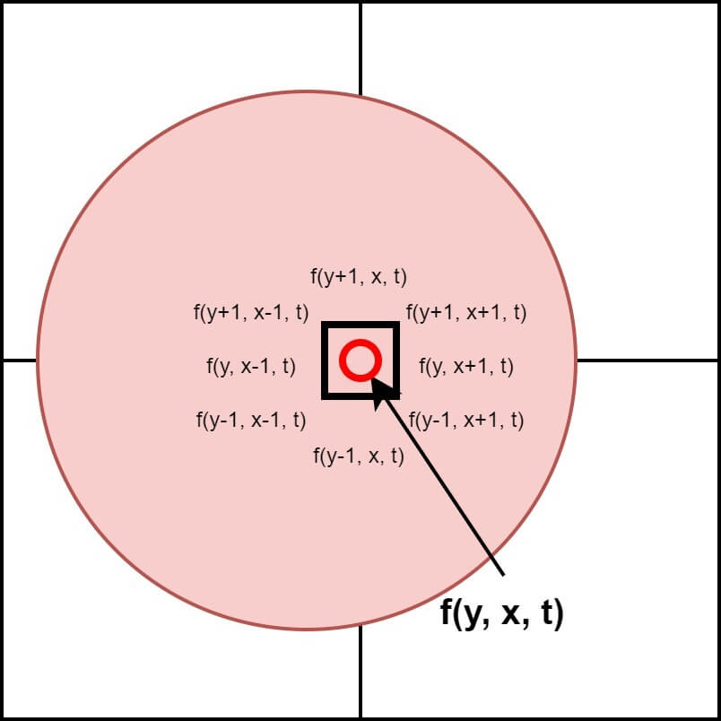
When we look at a specific point in an image, there is a high probability that adjacent pixels also have similar values. Although the example may be a bit messy, if we look at the hand touching the mouse right now, we can find such consistency. Adjacent pixels of the skin color have a similar color. This consistency in the image is used in various fields, and the easiest field to encounter is Edge Detection. Areas where the difference between adjacent pixels is small are likely to be the same object, and areas where the difference is large are likely to be the boundary between objects. Figure 1 is a concept figure of image coherence.
2.1.2. Time Coherence
When we view an image, objects move continuously. If the FPS (Frame Per Second) is sufficiently high, then objects that can teleport or change direction without delay in 180 degrees can be a counterexample to this post. If you have such examples, please leave a rebuttal comment with a reference URL, and I would appreciate it (you may even see the author in the news soon).
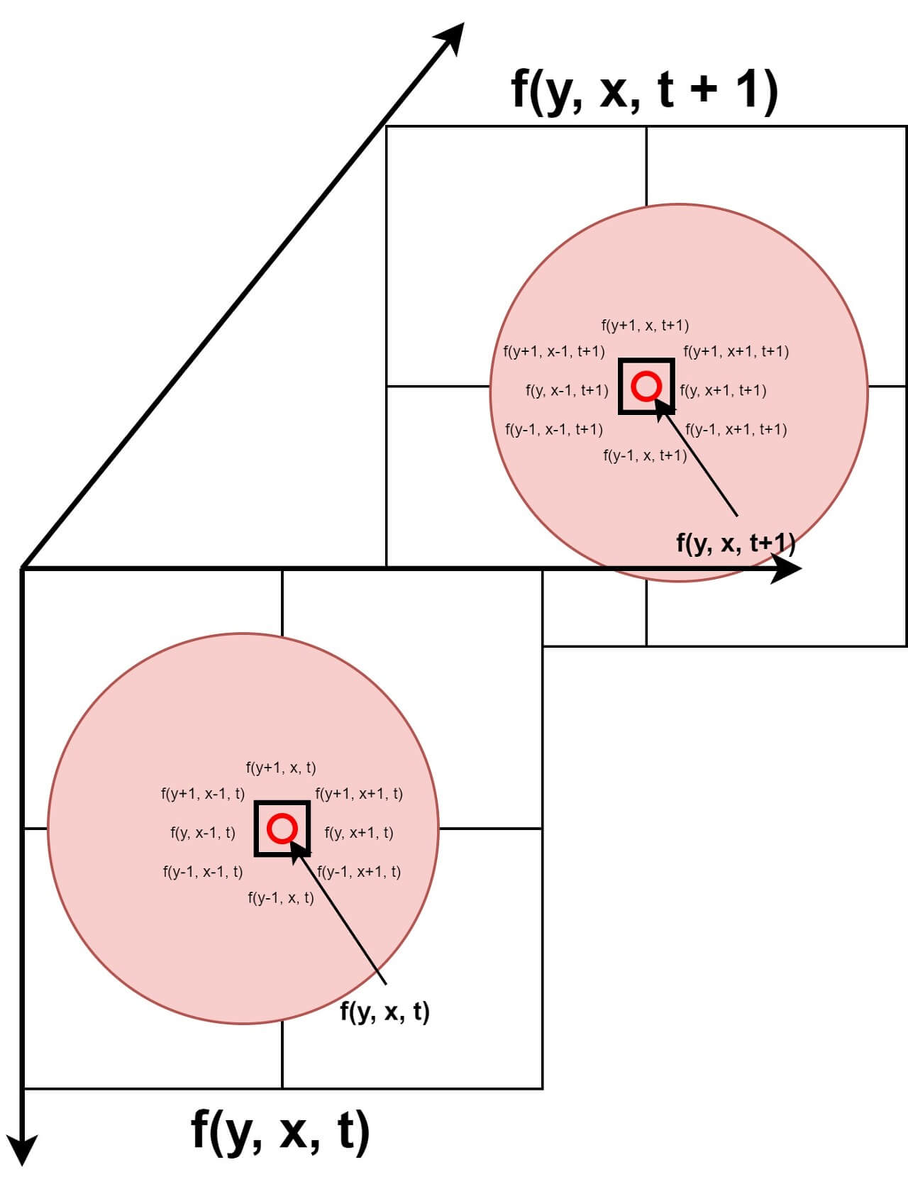
In other words, for a large change to occur, small changes must precede it. This means that if the pixel value at time t is $f(y,x,t)$, then $f(y, x, t+1)$ is likely to be the same or very similar. If the values are the same, it can be inferred that there was no movement. By utilizing this feature, basic segmentation can be performed. The difference between two images can be used to extract only the objects with large changes. This temporal consistency becomes a very important clue in Optical Flow. Figure 2 is a concept figure of time coherence.
2.2. Conclusion
In this chapter, we have discovered clues for calculating optical flow from a computer vision perspective. However, the most important thing is missing. So, what is Optical Flow? It's a natural question that should come to mind. In this chapter, intentionally, the definition of Optical Flow is not mentioned. It may have been perceived as "something to calculate the motion of objects." But is it possible for a computer to calculate the motion of objects like humans do? In the next chapter, we will cover what Optical Flow is. Is it really about calculating the motion of objects?
3. Motion Field vs Optical Flow
In the previous chapter, we found clues for calculating Optical Flow from a computer vision perspective. More precisely, we found clues to enable a computer to perceive the motion of an object like a human does. But does this mean that calculating Optical Flow is all that is left? Can a computer truly perceive the motion of objects like humans do?
In this chapter, we will compare Motion Field and Optical Flow, which is named after the motion of objects. Surprisingly, Optical Flow does not represent the motion of objects. So, what exactly is it? Let's first take a look at Motion Field, which represents the motion of objects.
3.1. Motion Field
Our friendly neighbor Wikipedia defines Motion Field as follows:
In computer vision the motion field is an ideal representation of 3D motion as it is projected onto a camera image.(...) The motion field is an ideal description of the projected 3D motion in the sense that it can be formally defined but in practice it is normally only possible to determine an approximation of the motion field from the image data.
Motion field - Wikipedia
From Wikipedia, the free encyclopedia In computer vision the motion field is an ideal representation of 3D motion as it is projected onto a camera image. Given a simplified camera model, each point ( y 1 , y 2 ) {\displaystyle (y_{1},y_{2})} in the image i
en.wikipedia.org
In short, Motion Field is an ideal representation of 3D motion as it is projected onto a camera image in computer vision. It captures all the movements of objects. The following figure shows an ideal Motion Field.
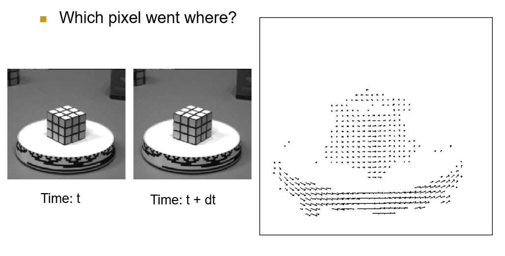
The terms "ideal" and "in practice" in the definition of the Motion Field on Wikipedia suggest that it is an idealized representation of 3D motion projected onto a camera image, and that while it can be formally defined, in practice it is often only possible to determine an approximation of the motion field from image data. In other words, it is impossible to accurately reproduce the motion field from 2D images or videos that we commonly encounter, unless using a holographic 3D point cloud.

There are several reasons for this, but to put it simply, it is because of the difference in dimensions as shown in the figure 4. Actual motion occurs in 3D space. However, the images or videos that we need to obtain a motion field from are 2D data. As the dimensions are reduced, numerous vectors in 3D space are projected onto 2D space, causing overlapping as shown in the figure. As a result, a significant amount of information is lost and distortion occurs. It is already difficult to capture things as they are, and attempting to capture all motion is ambitious.
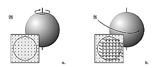
Due to this information loss, we cannot accurately obtain the Motion Field in real-world images. The most representative example is errors that occur in the rotation of objects and light sources, as seen in the above image. The image on the left shows an example where actual motion (rotation) occurred, but there appears to be no change in the image. Conversely, the image on the right shows an example where there was actually no motion, but changes in brightness occurred due to the movement of the light source, making it appear as if there was a change in the image. In other words, the problem arises when there is actual movement but no motion vector occurs (FN) or when there is no actual movement but a motion vector occurs (FP). Through this example, we can understand what Optical Flow is. Optical Flow is not strictly speaking a method for capturing the movement of objects. So what is it?
3.2. Optical Flow
Again, Our friendly neighbor Wikipedia defines Optical Flow as follows:
Optical Flow or optic flow is the pattern of apparent motion of objects, surfaces, and edges in a visual scene caused by the relative motion between an observer and a scene.
Actually, this sentence is not easy to understand. To express it accurately, it is not easy to know what the differences are compared to the Motion Field. The reason is that this definition lacks the "How". Conceptually, it is a major cause of confusion because there is little difference between it and the Motion Field. Therefore, I prefers the second definition explained by Wikipedia, which includes the "How".
Optical Flow can also be defined as the distribution of apparent velocities of movement of brightness pattern in an image.
Optical flow - Wikipedia
From Wikipedia, the free encyclopedia Pattern of motion in a visual scene due to relative motion of the observer The optic flow experienced by a rotating observer (in this case a fly). The direction and magnitude of optic flow at each location is represent
en.wikipedia.org
Optical Flow is the process of capturing changes in image frames by considering only brightness patterns, or changes in luminance. In an image, luminance changes lead to variations in pixel values, and by analyzing the difference between the previous and current frames and the relationship between the current pixel value and its surrounding pixels, the motion of each pixel can be approximated. Optical Flow does not explicitly calculate motion, but by computing changes in luminance caused by motion, it implicitly generates a map that can serve as a Motion Field.
The reason for separating Optical Flow from Motion Field is that Motion Field is not an accurate concept and can limit the scope of calculating motion. Optical Flow, which generates a Flow Map based only on changes in luminance, is an independent estimation method that does not attempt to detect objects or reflect their motion. This aspect is what sparked the strong interest of me, who specializes in signal processing.
3.3. Conclusion
In this chapter, we have looked at the concept of Optical Flow. In the next chapter, we will examine what conditions are necessary to actually calculate Optical Flow. As a hint, the concept of Coherence that we discussed in the previous chapter also appears here in the same way, except the terms are changed to Spatial Coherence and Temporal Persistence.
4. Optical Flow Constraint Equation (OFC)
In the previous chapter, we learned about what Optical Flow is. We also discussed the significant loss of information that occurs when compressing from 3D to 2D. To overcome this problem, Optical Flow makes several assumptions. The coherence concept we covered in the first chapter reappears here, but with a different name.
4.1. Assumptions
In order to calculate the 3D motion from an image compressed into 2D, we need to make assumptions. This must be done within the range that does not distort reality, and it should serve as an important clue to solving the problem.
4.1.1. Brightness is constant

Bright Constancy is an assumption that corresponds to the Image Coherence discussed in the first chapter. It assumes that in an image, a specific point, that is a pixel, and its neighboring pixels have the same color or brightness. In computer vision, color/brightness is represented by pixel values, so ultimately neighboring pixels have the same value.
However, for this assumption to hold true perfectly, it should be assumed that there are no changes in lighting. Additionally, changes in the angle between the object and the light source should not result in differences in brightness. In reality, it is impossible to create such conditions. To use Optical Flow in the real world, it must follow the laws of the real world. Fortunately, in practice, this assumption cannot be perfectly satisfied, but the errors can be accommodated by using a threshold to accept the degree of error that can be tolerated. Thanks to this, we can use important assumptions to design Optical Flow algorithms.
4.1.2. Motion is small

Small Motion is the assumption that corresponds to Time Coherence discussed in the first chapter. Large changes require small changes to precede them. The Optical Flow we are dealing with assumes small changes because it deals with changes between two consecutive frames.
In two consecutive frames, the same pixel of an object has the same brightness/color (i.e., the pixel values are the same or similar).
These two assumptions can be expressed as above, and they are the most important assumptions for calculating Optical Flow, so it is important to keep them in mind. In fact, if you think about it for a moment, it is a very obvious proposition. However, as with many assumptions in computer vision, it is a process of assuming the obvious to solve problems.
4.2. Optical Flow Constraint
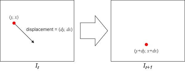
At time $t$, let's call the intensity of a point $(y, x)$ in the image as $I(y, x, t)$, and its value at $t+1(=t+dt)$ as $I(y+dy, x+dx, t+dt)$. Applying the first assumption, Brightness Constancy, we can derive the A equation below.
$$I(y,x,t)=I(y+dy,x+dx,t+dt)\Rightarrow A$$
If we apply Taylor series (expansion) to the right-hand side of the equation, we get the B equation as follows.
The omitted terms are second-order or higher-order terms. As these terms have a significantly smaller impact than the first-order term when $dy$ and $dx$ are sufficiently small due to the second assumption, Small Motion, and the time interval between two consecutive frames, $dt$, is sufficiently small, we can omit them completely.
However, it is not possible to define the exact value of a sufficiently small time interval, $dt$. It is a value that allows $dy$ and $dx$ to remain sufficiently small. Typically, if the movement of an object can be captured within a few pixels, it is considered a sufficiently small value. Therefore, what is important is not just the time interval, but also the amount of movement during that time interval.
Returning to the main topic, substituting the simplified B equation obtained under the assumption of a sufficiently small time interval into the A equation yields the following equation.
$$I(y,x,t)=I(y,x,t)+\frac{\partial I}{\partial y}dy+\frac{\partial I}{\partial x}dx+\frac{\partial I}{\partial t}dt+\cdots \Rightarrow B\,in\,A$$
If we simplify the previous equation a little more, we can get the desired form. The following equation finally allows us to focus on the change. While there is a method to derive this equation directly from the Taylor expansion through Brightness Constancy, we have shown the step-by-step derivation from the beginning for better understanding.
$$\frac{\partial I}{\partial y}dy+\frac{\partial I}{\partial x}dx+\frac{\partial I}{\partial t}dt=0$$
If we divide both sides of the equation by $dt$, it can be expressed as follows.
$$\frac{\partial I}{\partial y}\frac{\mathrm{d} y}{\mathrm{d} t}+\frac{\partial I}{\partial x}\frac{\mathrm{d} x}{\mathrm{d} t}+\frac{\partial I}{\partial t}=0,\quad I_yv+I_xuI_t=0$$
The second equation is a simplified version of the first equation, where each term has its own meaning. This equation is called the Optical Flow Constraint Equation, OFC for short, and sometimes also referred to as the Gradient Constraint Equation. Most Gradient-based Optical Flow algorithms are derived from this equation. However, this equation alone cannot calculate Optical Flow or Motion Vectors, and the reason for this is as follows.
4.3. Apperture Problem
Let's take a closer look at the OFC. Before examining the meanings of each term, let's separate them into variables and constants. The terms expressed by partial derivatives are constants that are determined dependently if the position and value of the pixel for which Optical Flow is to be measured are fixed. Therefore, the partial derivatives are constants, and the remaining terms expressed by derivatives can be viewed as variables. If you've followed this perfectly so far, you can discover a big problem. Is something weird? Isn't the equation weird? Brilliant! That's a great question. The above equation is weird. No, to be precise, it is insufficient. Let's first understand the meanings of the OFC terms.
4.3.1. Constants
$$\left ( \frac{\partial I}{\partial y},\frac{\partial I}{\partial x}\right )\Rightarrow Gradient\,\, Vector,\quad \frac{\partial I}{\partial t}=I(x,y,t+1)-I(x,y,t)$$
4.3.2. Variables
$$\left ( \frac{\mathrm{d} y}{\mathrm{d} t},\frac{\mathrm{d} x}{\mathrm{d} t} \right )\Rightarrow Motion\,\,Vector,\quad\frac{\mathrm{d} y}{\mathrm{d} t}=v,\quad\frac{\mathrm{d} x}{\mathrm{d} t}=u$$
The three vectors that make up the constant term are values measured from the image, and (v, u) must be calculated using these values. Here, a strange point is discovered. There is only one equation, but there are two unknowns to be solved... The equation is insufficient. In other words, the Optical Flow Constraint Equation cannot uniquely determine the Motion Vector. This means that without other assumptions, it is impossible to determine the motion at a single point. This problem is known by various names such as the "pinhole problem" or "aperture problem."
4.4. Conclusion
In this chapter, we looked at the important assumptions and equations, including the Optical Flow Constraint Equation (OFC), for calculating Optical Flow. You may have felt frustrated after following along diligently but realizing that we can't determine the Motion Vector with just one equation. However, as an Algorithm Engineer, if the equation is incomplete, we can add additional assumptions to fill it out. In fact, in the next chapter, we will explore the more commonly known Lucas-Kanade and Horn-Shunck algorithms, which add conditions to find solutions to equations and determine the Motion Vector. Let's first take a closer look at the Lucas-Kanade algorithm.
5. Lucas-Kanade Algorithm, Part 1
The Optical Flow Constraint Equation (OFC) we derived earlier is insufficient to actually compute the Optical Flow. With two unknowns and only one equation, we cannot determine a solution. Therefore, we need to add assumptions, and the first method we will discuss is the Lucas-Kanade method. We will present the added assumption, the computation of Optical Flow, and the advantages and disadvantages in that order.
5.1. Assumption
The assumption added in the Lucas-Kanade Method highlights the characteristics of the algorithm well. The Optical Flow of the $n \times n$ window $N(y, x)$ created around the pixel $(y, x)$ are all the same. That is, the pixels inside the window move in the same direction, and therefore have the same Motion Vector values. This indicates that the algorithm finds the solution of the Optical Flow problem using a local approach. With the addition of the new assumption, the Lucas-Kanade Algorithm now has a total of three assumptions, in addition to the two existing ones:
- Brightness is constant
- Motion is Small
- Flow is essentially constant in a local neighborhood of the pixel
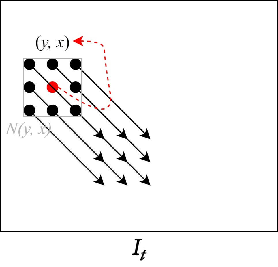
The OFC can be modified with the addition of this new assumption. The window size in this case is the number of pixels included in $N(y, x)$. The modified OFC with the new assumption is as follows.
$$\frac{\partial I(y_{i},x_{i})}{\partial y}v+\frac{\partial I(y_{i},x_{i})}{\partial x}u+\frac{\partial I(y_{i},x_i)}{\partial t}=0,{\quad}(y_i,x_i)\in N(y,x)$$
To transform the above equation into a matrix form, we can expand it as follows. Let $p$ be the center point of the window, and let $q$ be the neighboring pixels of $p$, although they do not appear in the following equation.
$$I_x(q_1)V_x+I_y(q_1)V_y=-I_t(q_1)$$
$$I_x(q_2)V_x+I_y(q_2)V_y=-I_t(q_2)$$
$$\vdots$$
$$I_x(q_n)V_x+I_y(q_n)V_y=-I_t(q_n) $$
Surprisingly, unlike the previous OFC that was insufficient with 2 unknowns and 1 equation, this time the equations overflow. There are $n$ equations depending on the Window Size, so there is no problem in determining the Optical Flow. Now let's convert the above equation into matrix calculation form of $Av = b$.
$$A=\begin{bmatrix}
I_x(q_1) & I_y(q_1) \\
I_x(q_2) & I_y(q_2) \\
\vdots & \vdots \\
I_x(q_n) & I_y(q_n) \\
\end{bmatrix},\quad v=\begin{bmatrix}
V_x \\V_y
\end{bmatrix},\quad b=\begin{bmatrix}
-I_t(q_1)\\
-I_t(q_2)\\
\vdots\\
-I_t(q_n)\\
\end{bmatrix}$$
After converting to matrix form, it is more intuitive that there are too many equations compared to the required number. To reduce the number of equations to the necessary minimum, we can use the Least Squares Principle. We can obtain the Motion Vector by transforming the equation into a form that is a function of $v$, as shown below.
$$A^{T}Av=A^Tb \quad \Rightarrow \quad v=(A^TA)^{-1}A^Tb$$
$$\begin{bmatrix}
V_x \\V_y
\end{bmatrix}=\begin{bmatrix}
\sum _iI_x(q_i)^2&\sum _iI_x(q_i)I_y(q_i) \\
\sum _iI_y(q_i)I_x(q_i)& \sum _iIy(q_i)^2 \\
\end{bmatrix}^{-1}\begin{bmatrix}
-\sum _iI_x(q_i)I_t(q_i) \\ -\sum _iI_y(q_i)I_t(q_i)
\end{bmatrix}$$
5.2. Pros and Cons
Finally, we learned a way to calculate Optical Flow. However, the Lucas-Kanade Method is just one of the methods to calculate Optical Flow, as we can create various algorithms by adding different assumptions to the basic OFC. Each method has its own advantages and disadvantages, so it is important to choose the algorithm that is suitable for the situation. So what are the pros and cons of Lucas-Kanade? If you have some experience in Computer Vision, you may immediately think of the answer. The result is highly dependent on the Window Size! If the Window Size is large, the operation will be fast but inaccurate, and vice versa. That's right. The rest are pros and cons from an Optical Flow perspective, so you don't have to feel overwhelmed if you don't immediately understand them. It's natural to not know everything.
- Pros
- It belongs to Sparse Optical Flow and uses points with prominent features such as edges, resulting in low computation.
- Cons
- The Window Size is generally small, so it cannot calculate movements larger than the window.
- Since it calculates Optical Flow based on a specific point, the accuracy is lower than that of Dense Optical Flow, which calculates globally.
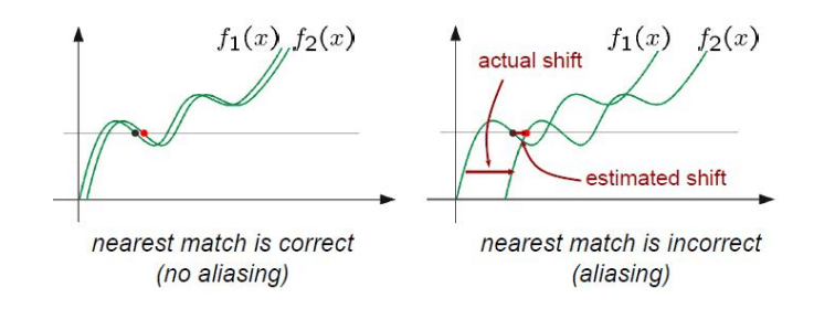
The part that may be difficult to understand in the cons is probably when there are movements larger than the window. Since it is based on value tracking, Isn't it okay even if the movement is large? The problem is that window-based algorithms do not consider outside the window. Therefore, aliasing occurs in this case, resulting in distortion as shown below.
5.3. Conclusion
In this chapter, we learned how to calculate Optical Flow using the Lucas-Kanade Algorithm and its additional assumptions. We also learned that LK is not a perfect method, as it has its own advantages and disadvantages. Algorithm engineers continue to work on improving this method when problems arise. There are numerous ideas to improve LK, including using weights that are common in window-based algorithms to improve accuracy and proposed methods to deal with Big Motion, which we will discuss in the next post. Additionally, we will mention the persistent problems of Sparse Optical Flow that were not covered in this post. Through this process, we will experience the extension of the concepts previously mentioned.
6. Lucas-Kanade Algorith, Part 2
In the previous chapter, we looked at how to calculate optical flow using the assumptions added to the Lucas-Kanade algorithm. In this chapter, we will discuss methods to improve the accuracy of the Lucas-Kanade algorithm using weights and techniques proposed to handle big motions. Additionally, we will mention the inherent issues of sparse optical flow that were not covered in the previous chapter.
6.1. Weighted Window
The Lucas-Kanade Algorithm is designed based on a window. Pixels within the same window have the same Optical Flow value. Although it is an assumption, it is not questioned much. However, if we think a little more, it is not very realistic, especially at the edges where there can be significant errors. Weighted windows provide some correction to the Lucas-Kanade assumption to make it more practical. The closer to the center of the window, the larger the weight, and the pixels within the window can have different values. Gaussian weights are commonly used.
$$A^{T}WAv=A^TWb \quad \Rightarrow \quad v=(A^TWA)^{-1}A^TWb$$
$$\begin{bmatrix}
V_x \\V_y
\end{bmatrix}=\begin{bmatrix}
\sum _iw_iI_x(q_i)^2&\sum _iw_iI_x(q_i)I_y(q_i) \\
\sum _iw_iI_y(q_i)I_x(q_i)& \sum _iw_iIy(q_i)^2 \\
\end{bmatrix}^{-1}\begin{bmatrix}
-\sum _iw_iI_x(q_i)I_t(q_i) \\ -\sum _iw_iI_y(q_i)I_t(q_i)
\end{bmatrix}$$
The above equation is the result of adding weight to the conventional Lucas-Kanade expansion. The equation using Gaussian weight uses the Gaussian function value of the distance between the i-th $p$ and $q$ values to determine the i-th $w$ value.
6.2. Coarse to Fine Strategy (Image Pyramid)
As mentioned in the previous chapter, the Lucas-Kanade Algorithm is vulnerable to big motion (large displacement). Why is that? Do you remember that Short Displacement was assumed for Taylor Approximation? It would be a natural answer. However, if we leave it vulnerable to big motion, it would be difficult to use in the real world. Therefore, a little trick is applied. In traditional image processing, it is called the Image Pyramid technique, while in recent computer vision fields using deep learning, it is called the Coarse to Fine Strategy.
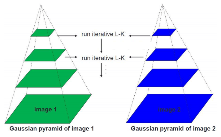
Image Pyramid (Coarse to Fine Strategy) is a technique that transforms an image from a low-resolution (down-scaled) to a high-resolution (up-scaled) image, widening the convergence of algorithms that operate on the entire image domain. By utilizing this technique, large displacements in reality can appear as short displacements. Even if there are movements of more than 50 pixels in the original image, they can be minimized to within 5 pixels by down-scaling.
This method measures short displacements in the down-scaled image and obtains the final flow map by up-scaling to the original image. However, this method has the problem of error propagation because a lot of information is lost during the down-scaling process, and errors generated in the low-resolution image are not corrected but instead maintained during the up-scaling process.

7. EpicFlow (CVPR 2015)
In the previous chapter, we talked about improving the accuracy of the Lucas-Kanade Algorithm through weighting and proposed methods to address Big Motion. We have so far discussed the most representative Handcrafted method, Lucas-Kanade, and in this post, we will discuss EpicFlow, which is considered the essence of Handcrafted techniques (my personal opinion). This will be the last time we mention Handcrafted techniques (Horn-Schunck, etc. will be covered if I have time). The reason for covering EpicFlow last is because it is often cited as a benchmark for comparison with Deep Learning-based techniques that will be introduced in the future.
7.1. Architecture
EpicFlow is a paper presented at CVPR2015. It added something to the Coarse-to-Fine technique used in Lucas-Kanade and similar ideas to improve performance. You can easily understand this idea by looking at the picture.

EpicFlow goes through three major steps to obtain a Flow Map. First, it uses a matching algorithm to obtain a matching sparse set between two images. The algorithm used for this step is the one that has the best performance (state-of-the-art). Then, it obtains a precise Flow Map through sparse-to-dense interpolation that corresponds to Coarse-to-Fine. Finally, it uses energy minimization to obtain the final Optical Flow.
The above explanation contains too many proper nouns, and the description is somewhat unfriendly, to the extent that it is easier to understand the idea through the figure. Therefore, I will explain it step by step. Of course, this post is not intended to master EpicFlow. On the contrary, it is closer to understanding the concept of EpicFlow, which is the essence of Handcrafted techniques and a counterpart to Deep Learning techniques in the future. Therefore, I will not provide too detailed an explanation, so please understand.
7.2. Sparse set of Matches
The first step of EpicFlow is to extract matching pairs between two frames. As mentioned, any state of the art matching algorithm can be used. In experiments, the Deep Matching and Subset of an estimated nearest-neighbor field methods were used. Obtaining matching pairs means matching features between the two images.
Feature descriptor is an example of a matching algorithm, which matches characteristic points between two images with different viewpoints or affine transformations. In other words, it finds the same points in two different images, and it extracts sparse matching pairs through characteristic points such as edges, rather than matching all pixels. For more detailed information on this, I recommend referring to the blog link in the references.

7.3. Interpolation Method
The second step of EpicFlow is to estimate a dense Flow Map through an interpolation process using the matching pairs obtained in the first step. EpicFlow proposes two methods for this:
- Nadaraya-Watson (NW) Estimation
- Locally-weighted Affine (LA) Estimation
In addition, the number of matching pairs used in the interpolation is limited by using local interpolation and only considering the K-nearest neighbors. This improves the computational speed.
Finally, the interpolation results are refined using Energy Minimization to obtain a final Optical Flow with sharper edge points. However, this post will not cover Energy Minimization in detail (it may be covered later along with the Horn-Schunk algorithm if I have time).
7.4. Edge-preserving Distance
Now that most of the EpicFlow architecture have been addressed, the remaining one is the Edge Map obtained as a result of contouring. Why is the Edge Map used in EpicFlow? As we learned in previous chapters, the Coarse-to-Fine technique was used to compensate for the Lucas-Kanade Algorithm's vulnerability to Large Displacement. However, this method also had an Error Propagation problem, where errors from coarser levels propagate to higher levels.
Sparse-to-Dense Interpolation addressed this issue by utilizing only some of the matching results. However, this process causes a significant loss of information, and selecting sparse feature points is important to achieve a uniform result or an expected value. The Edge Map was proposed here, as the boundaries of new motions are typically observed at the edges of the image. Therefore, EpicFlow preserves the motion boundaries, namely the Edge Map, to calculate Optical Flow.
When using the typical Euclidean Distance, the Flow Map is significantly affected by the surrounding background in the Edge region, causing problems with the result being distorted during interpolation. Therefore, the Geodesic Distance (Edge-aware Distance) is utilized. Geodesic Distance is computationally intensive, so it takes a long time. Therefore, an Approximation is used, but we will not cover it in this chapter. Instead, let's learn about the difference between Geodesic Distance and Euclidean Distance in figure 13.
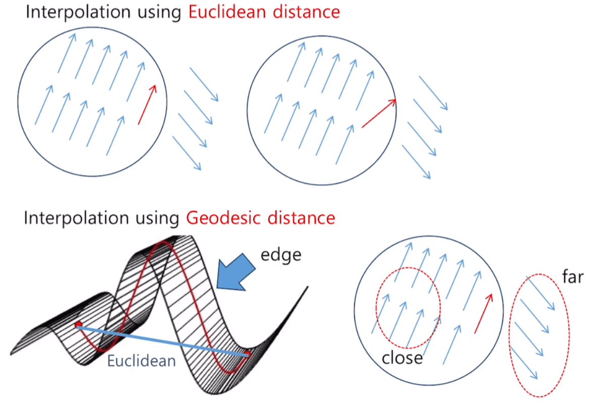
If Euclidean distance is used in Coarse-to-Fine/Sparse-to-Dense Interpolation, as in the figure 13, it is greatly affected by the background. As a result, the vectors at the edge part have values different from the intended ones. On the other hand, using Geodesic distance results in little to no damage to Optical Flow during interpolation.
The figure in the bottom of figure 13 shows a side view of the Edge Map. With Euclidean distance, as shown in the blue line, straight-line distance is used, so it does not distinguish between vectors outside and inside the edge. On the other hand, Geodesic distance considers the Edge Map when measuring distance, resulting in a significant detour effect when crossing the edge. Therefore, it helps to maintain similar tendencies among vectors in the same Edge Map.
7.5. Conclusion
Next, we will cover FlowNet, which began measuring optical flow using deep learning. It was a more interesting paper that was released in the same year as EpicFlow, and FlowNet 2.0, which improved performance, was also used for my research topic.
However, before we touch deep learning methods, we will gonna touch two basic knowledge of current Optical Flow research. First one is about flow map, which is used for representing the result vectors. Second one is the dataset for Optical Flow in deep learning.
8. Flow Map (Vector/HSV)
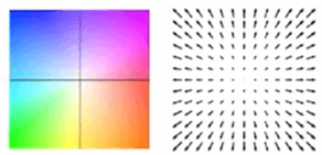
In the previous chapter, we covered Epicflow as the last Handcrafted method. While discussing Epicflow, we introduced a different type of Flow Map without much explanation. Up until now, the Flow Map (Vector Map) has been represented by vectors (arrows). However, even if we densely calculate Optical Flow using vectors, we can only draw a sparse Flow Map using vectors.
On the other hand, if we represent vectors with colors, as shown in the image below, we can represent vectors for all pixels. In Optical Flow, we use an HSV color map rather than the commonly used RGB.

8.1. HSV Vector Map
As mentioned in the introduction, Vector Maps have poor visual appeal and cannot be represented densely. Therefore, Optical Flow Maps are often represented using an HSV Map. First, let's take a look at what an HSV Map is. The difference between an HSV Color Map and the RGB Color Map that we commonly use is as follows:
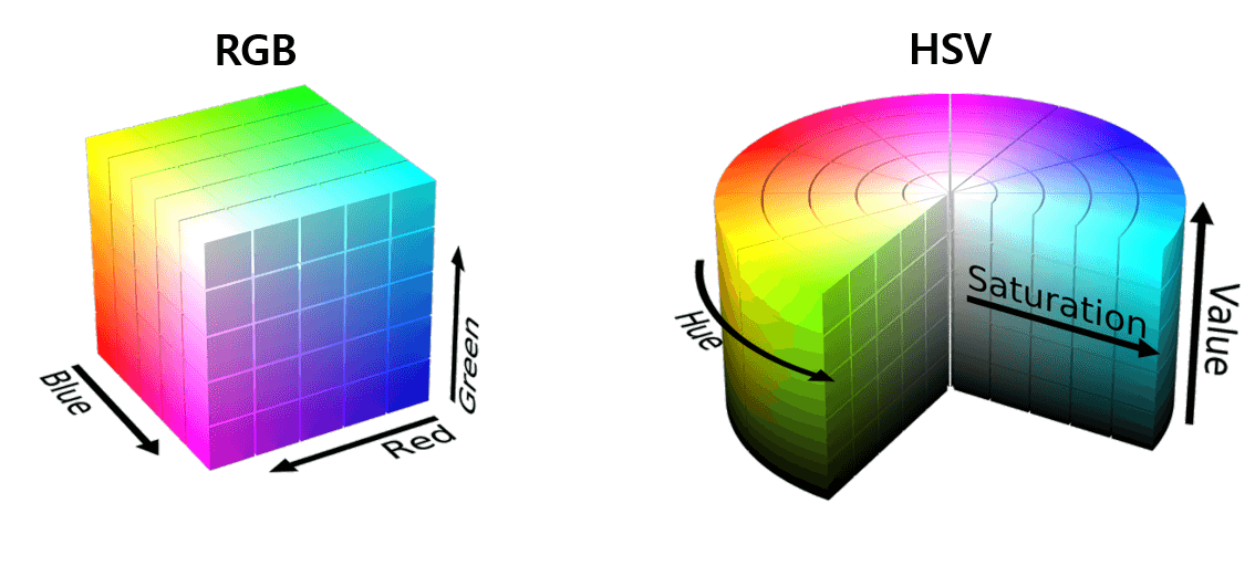
Unlike RGB, which combines Red (R), Green (G), and Blue (B) to represent all colors, HSV uses a combination of Hue (H), Saturation (S), and Value (V) to represent colors. Each component represents color, saturation, and brightness information, respectively. So how can we use HSV maps in a flow map? Each component of the HSV map plays the following roles:
- H (Hue): color information, direction of motion vectors
- S (Saturation): saturation information, size of motion vectors (darker colors mean larger vectors, lighter colors mean smaller vectors)
- V (Value): brightness information, not used in the flow map.
The following is a concept image that corresponds Vector Map to HSV Map.
9. Optical Flow Dataset
As deep learning-based optical flow algorithms have emerged, datasets have become a very important keyword. Optical flow is difficult to obtain ground truth for, and even if ground truth is obtained in the real world, the amount of data is very limited. In other computer vision fields such as object detection, data labeling is easy, making it relatively easy to solve these problems. However, the optical flow field still lacks in both quantity and quality.
Nevertheless, as always, humans have found solutions, and a revolutionary method has emerged in the optical flow field, which has become the industry standard. In the field of Optical Flow, there are mainly four types of datasets that are commonly used:
- Flying Chairs
- Flying Things 3D
- MPI-Sintel
- KITTI
To briefly introduce, Flying Chairs/Flying Things 3D are graphic (synthetic) datasets. Therefore, the input values become the labels and ground truth of Optical Flow. Despite being an artificial dataset, it is widely used and has become a standard for training, thanks to the ease of labeling.
On the other hand, MPI-Sintel/KITTI are real datasets. However, due to the nature of Optical Flow, it is difficult to obtain a large amount of ground truth data, so only a small amount of data is provided. Therefore, it is used for fine-tuning and testing.
To summarize the above explanations, the training and testing process of an Optical Flow model is as follows:
- Training (scheduling): Flying Chairs/Flying Things 3D
- Training (fine-tuning before test): Flying Things 3D/MPI-Sintel/KITTI
- Testing: MPI-Sintel/KITTI
9.1. Flying Chairs/Flying Things 3D
The details about those datasets will be introduced in next chapters, FlowNet and FlowNet 2.0. So, we will talk about the details later. Now, here is download links as follows:
- Flying Chairs
Computer Vision Group, Freiburg
Datasets Optical Flow Datasets: FlyingChairs, ChairsSDHom The "Flying Chairs" Dataset The "Flying Chairs" are a synthetic dataset with optical flow ground truth. It consists of 22872 image pairs and corresponding flow fields. Images show renderings of 3D c
lmb.informatik.uni-freiburg.de
- Flying Things 3D
Computer Vision Group, Freiburg
Datasets Scene Flow Datasets: FlyingThings3D, Driving, Monkaa This dataset collection has been used to train convolutional networks in our CVPR 2016 paper A Large Dataset to Train Convolutional Networks for Disparity, Optical Flow, and Scene Flow Estimatio
lmb.informatik.uni-freiburg.de
9.2. MPI-Sintel
MPI (Max Planck Institute) Sintel is a dataset extracted from the 3D short animation "Sintel". It consists of a total of 1064 images, and the site introduces the features of the dataset as follows:
- Very long Sequences
- Large Motions
- Specular Reflections
- Motion Blur
- Defocus Blur
- Atmospheric Effects
The official site is http://sintel.is.tue.mpg.de/ and you can download the dataset from http://sintel.is.tue.mpg.de/downloads.
9.3. KITTI
The KITTI dataset is likely to be very familiar to those of you who work in Computer Vision. In particular, those who work on SLAM should be familiar with it. Surprisingly, the KITTI dataset includes a flow dataset specifically for Optical Flow. When I was studying Optical Flow, I was surprised to discover the flow dataset for the first time, since I had only used the odometry dataset when working on SLAM.
- KITTI 2015 (Optical Flow Evaluation 2015)
The KITTI Vision Benchmark Suite
When using this dataset in your research, we will be happy if you cite us: @ARTICLE{Menze2018JPRS, author = {Moritz Menze and Christian Heipke and Andreas Geiger}, title = {Object Scene Flow}, journal = {ISPRS Journal of Photogrammetry and Remote
www.cvlibs.net
10. FlowNet (ICCV 2015)
In the previous chapters, we looked at Handcrafted Optical Flow techniques. From now on, we will cover research on obtaining Optical Flow through Deep Learning. It all started with FlowNet, which was presented at ICCV 2015. Before FlowNet, there was a lack of research on hardware and Deep Learning, and the most important point was the lack of Optical Flow Groundtruth datasets required for learning. In this chapter, we will examine how FlowNet overcame these limitations.
FlowNet is an algorithm that uses supervised learning to estimate optical flow. It overcame the limitation of the lack of optical flow ground truth data for supervised learning by using its own method. This approach made a significant contribution to optical flow research, and we will cover it in the Dataset section.
FlowNet is an end-to-end CNN-based learning method. Since optical flow takes two images as input, it introduced a correlation layer to perform pixel-level localization for end-to-end learning.
Traditional handcrafted optical flow estimation methods such as Lucas-Kanade and Horn-Schunck manually set the algorithm's parameters without separate training. Therefore, performance differences may occur depending on the engineer's skill and understanding. However, FlowNet, which uses deep learning techniques, can minimize human intervention and solve such problems.
10.1. Dataset
Generating ground truth for optical flow estimation is a challenging task, as existing algorithms may have bias or inaccuracies. However, manually creating data for training may also result in an unsuitable format for machine learning. To address this issue, FlowNet created a synthetic dataset called Flying Chairs, which combines 3D chair images with Flicker DB. This allows for the creation of training data that is difficult to obtain in real life, while avoiding the limitations of manual data creation.

The Flying Chairs dataset proposed in FlowNet was not just an idea but actually succeeded in estimating optical flow. This demonstrated that a network trained on synthetic images can be applied to real-world images. Subsequently, many synthetic datasets, including Flying Chairs, have been widely used for learning in other optical flow research where real data is scarce.
10.2. Concept
To obtain optical flow between two frames, it inevitably requires two inputs. To learn in an end-to-end format with two input values, FlowNet proposes two methods. First, figure 17 is a basic concept image of FlowNet.
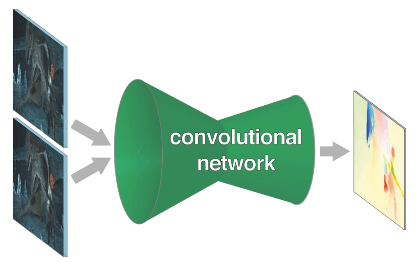
The Optical Flow is computed by training a CNN architecture in an End-to-End manner. Depending on the network architecture, there are two models: the FlowNetS, which is a generic architecture, and the FlowNetC, which uses the correlation of feature maps between the two input images. S and C stand for Simple and Corr (Correlation), respectively.
In addition, to achieve practical learning considering the computational complexity, pooling layers are used. This has the effect of combining information from a wide area, which I think is similar to the Coarse-to-Fine technique used in traditional Optical Flow methods.
Like the Coarse-to-Fine technique, a process of restoring the reduced resolution is necessary. In FlowNet, this process is performed by the Refinement layer, which acquires a pixel-wise Flow Map with the same resolution as the input images, resulting in a CNN-based End-to-End model.
10.3. Architecture
FlowNet proposes two architectures, FlowNetSimple (FlowNetS) and FlowNetCorr (FlowNetC), as shown in figure 18.
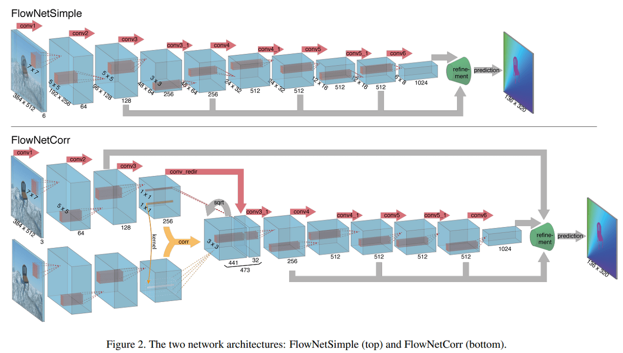
- FlowNetSimple
FlowNetSimple is a simpler network that concatenates two input images required for optical flow calculation into a single input channel of size 6. The subsequent network structure follows the traditional CNN architecture, and it is trained using supervised learning to enable the network to determine the optical flow extraction method on its own.
- FlowNetCorr
FlowNetCorr has a more complex structure compared to FlowNetSimple. The number of input channels is reduced to 3, indicating that there is no concatenation process. Instead, the input is divided into two input streams for the two input images. The input streams are identical in structure and each stream extracts the feature maps of the corresponding input image. The Correlation layer is used to merge these feature maps into a single representation. The authors of the paper refer to this feature map as the meaningful representations of the two images.
The question arises as to how the Correlation layer merges feature maps obtained through feature extraction rather than images. We will explore this in detail in the following chapter.
10.4. Correlation and Refinement Layer
FlowNet mostly follows a conventional CNN architecture, so it is not difficult to understand. However, the Correlation layer requires additional explanation. We will also provide an explanation of the Refinement layer, which is not usually seen in conventional CNN architectures.
- Correlation layer
The paper expresses the Correlation process using the following equation:
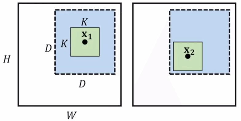
$$c(\mathbf{x_{1}}, \mathbf{x_2}))=\sum_{\mathbf{o}\in [-k,k]\times[-k,k]}\left<\mathbf{f_1(x_1+o),f_2(x_2+o)} \right>$$
First, we need to define $d, D, k, and K$ for correlation. This process is complex to express in words, so we will omit it and provide a link to the paper in the references for your reference. After defining the region, if we look at the correlation operation at the vector unit level, we can see that it can be viewed as the dot product between the vector at position $\mathbf{x_1}$ and the vector at position $\mathbf{x_2}$. Simply put, this is the process of stacking the resulting values obtained by taking the dot product of each element of the pre-defined patch and then summing them along the channel axis.
$$(w \times h \times D^2)$$
The output of the Correlation layer is a rectangular parallelepiped of the size of the above value. Figure 19 is an example illustration to help understand the Correlation layer.
- Refinement layer
The refinement layer is the final layer in FlowNet. Both FlowNetS and FlowNetC have refinement layers. First, let's examine the structure through figure 20.
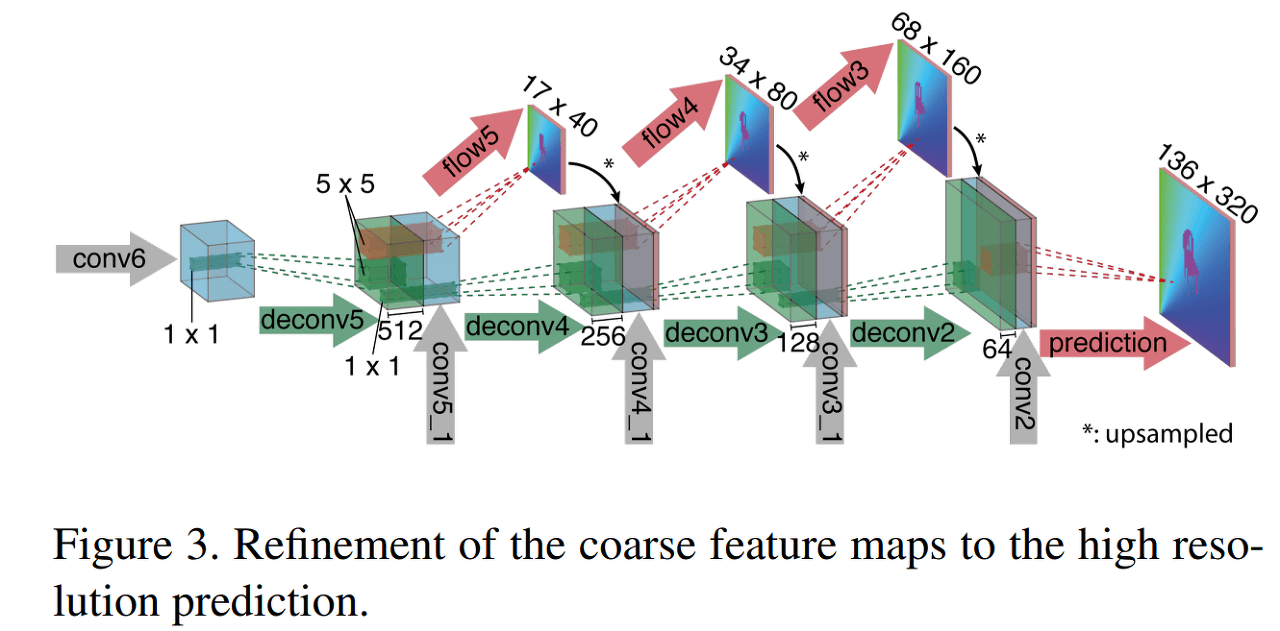
As shown in the figure, the Refinement layer is a structure that repeats Upsampling and Convolution. It also uses a concatenation method that concatenates the layers calculated in the front, such as conv5_1 and conv4_1, in between.
In addition, Flow Maps for intermediate results such as flow5 and flow4 are extracted, and the loss is calculated by comparing them with the Downsampling version of the Groundtruth image. Optical Flow often uses the EPE (End Point Error) Loss, which is the L2 Loss between the Estimated and Groundtruth values.
10.5. Contribution
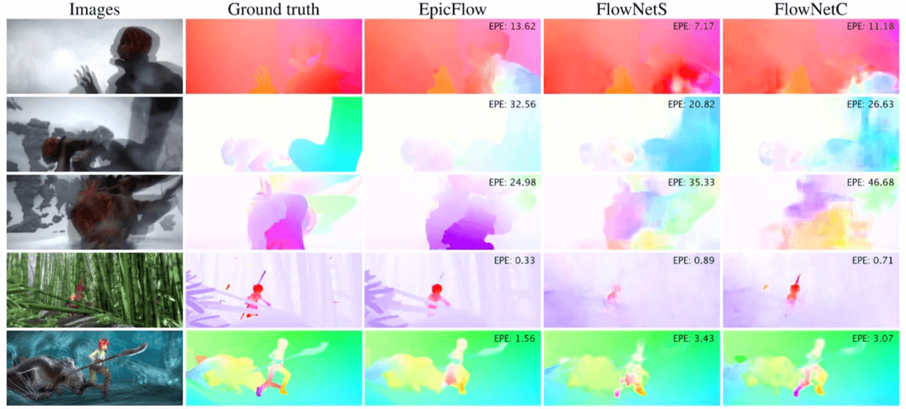
From the content written so far, FlowNet seemed like an innovative technique that would bring an end to handcrafted approaches. However, surprisingly, the performance of FlowNet did not turn out as good as expected.

FlowNet has sufficient contributions beyond being the end of handcrafted techniques, even though its performance is not as good as Epicflow, which is considered the pinnacle of handcrafted techniques, in terms of EPE. It has been confirmed that synthetic images can be used for training that is applicable to real-world scenarios. Additionally, the Flying Chairs Dataset, which is essential for DL-based Optical Flow research, was created. The calculation speed of Optical Flow, which was only possible with CPUs, was greatly improved by bringing it into the GPU domain.
Furthermore, with the release of FlowNet2.0 at CVPR 2017, it proved the significance of their direction for improving the performance of FlowNet. It is a meaningful paper that I was responsible for in my graduation research. FlowNet2.0 can be said to inherit everything from FlowNet. Therefore, a high level of understanding of FlowNet is essential.
11. FlowNet 2.0 (CVPR 2017)
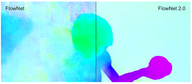
In the previous chapter, we covered FlowNet, the first DL-based Optical Flow algorithm. Despite having several important contributions, FlowNet fell behind in performance compared to the traditional handcrafted approach, EpicFlow. FlowNet2.0 is a network created to improve the performance of FlowNet.
In this chapter, we will focus on the key differences that FlowNet2.0 has compared to the previous version, that led to performance improvement.
11.1. Dataset
FlowNet2.0 pre-trained on the previously used Flying Chairs dataset and then further trained on the newly added FlyingThings3D (Things3D) dataset.
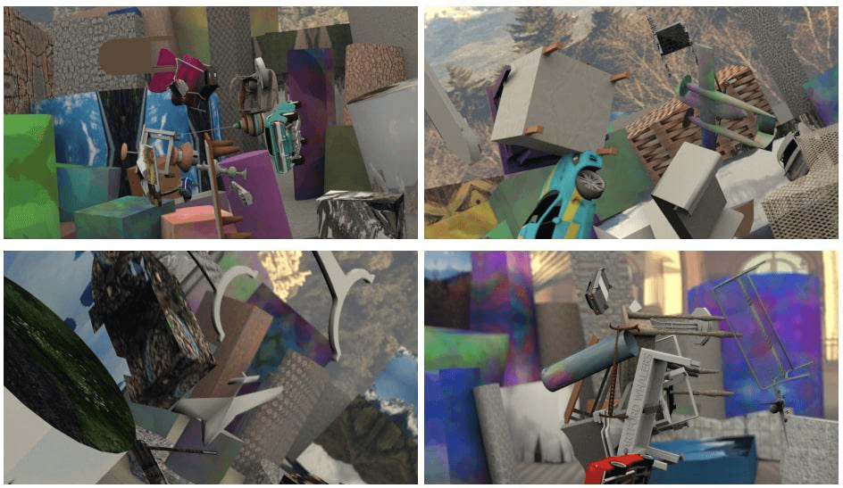
The paper expresses that the order of presenting training data with different properties matters. As a result, the paper suggests a method of pretraining with Chairs and then fine-tuning with the more real Things3D dataset.
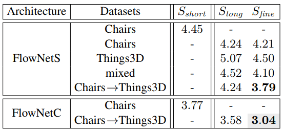
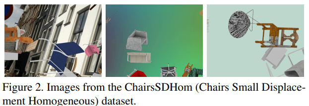
Also, more training was conducted compared to FlowNet, and additional training using the ChairsSDHom dataset was also carried out to improve Small Displacement performance. More details on this will be covered at the following chapters.
11.2. Architecture
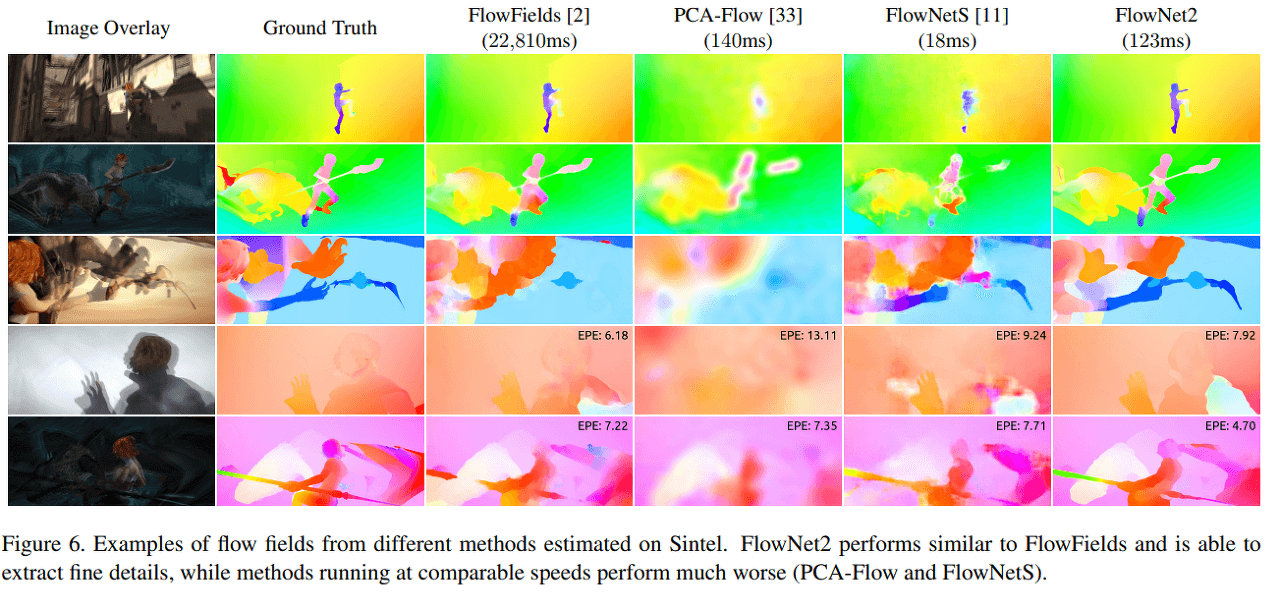
In the previous chapter, it was mentioned that FlowNet2.0 inherits everything from FlowNet. This can be understood from the network architecture. FlowNet2.0 improves performance by combining FlowNetS and FlowNetC proposed in FlowNet. Various combinations are presented in the paper, and the combination of FlowNetC + FlowNetS + FlowNetS showed the best performance.
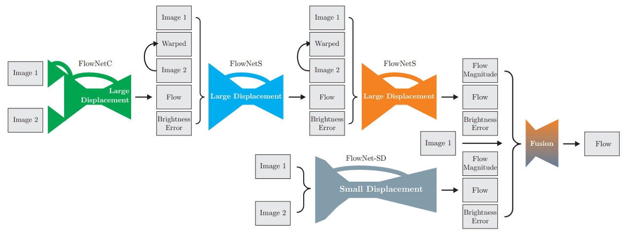
The technique of stacking networks to achieve better performance is quite common. However, FlowNet2.0 not only stopped there but also added something of its own - FlowNet-SD to address Small Displacement. This will be discussed in more detail later.
Ultimately, FlowNet2.0 acquires flow, flow magnitude, and brightness error from two models, FlowNet2-CSS-ft-sd and FlowNet2-SD. Each network corresponds to Large Displacement and Small Displacement, and the Fusion layer reflects both results to generate the final Flow Map.
11.2.1. FlowNet-SD
Although FlowNet was an optical flow algorithm, it had the advantage of being quite robust in the face of large displacements. However, it was surprisingly vulnerable in small displacements, making it difficult to apply in real-world problems. I have two possible explanations for this.
First, the dataset used to train FlowNet was biased toward large displacements. Deep learning is entirely dependent on the dataset, and since FlowNet used synthetic data instead of real-world data, it may have generated biased data. This seems plausible given that FlowNet-SD has somewhat addressed this issue.
Second, there are inherent limitations in the CNN structure. CNNs have an enormous computational load, which inevitably leads to the use of pooling layers. This can result in the loss of a significant amount of information as well as a decrease in resolution. This naturally leads to a similar effect to the Coarse-to-Fine technique and causes an error propagation problem. Additionally, since large movements are expressed by small pixels, there may be a significant effect of small movements being completely ignored.
Anyway, regardless of these personal opinions, FlowNet-SD first reduced the stride and made the feature map more sensitive to small changes when generating a feature map from FlowNetS. Additionally, to correspond to small displacements, it trained using ChairsSDHom dataset, which has smaller movements and follows the displacement histogram of UCF101.
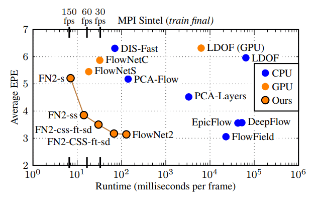
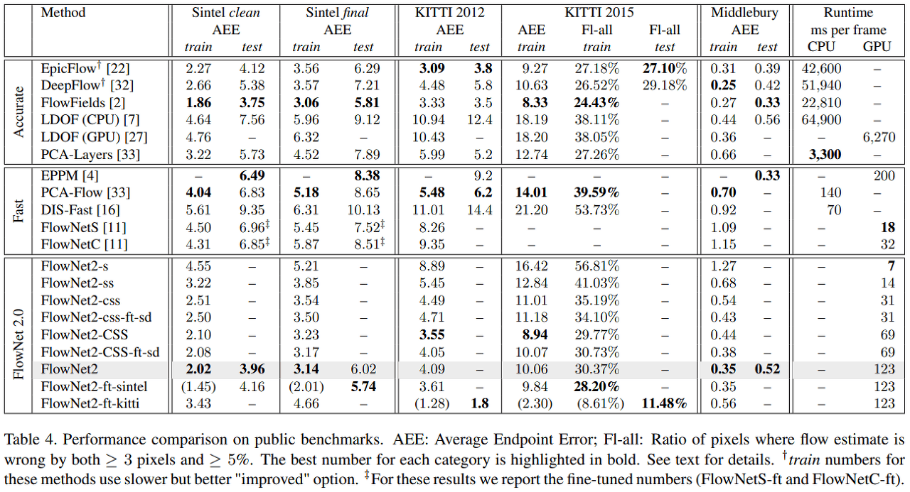
11.3. Result
12. PWC-Net (CVPR 2018)
In previous chapters, we covered the first DL-based Optical Flow algorithm, FlowNet, and its improved version, FlowNet2.0. In this chapter, we will discuss PWC-Net, which combines several techniques used in classical Optical Flow algorithms and applies them to a CNN model. PWC-Net can be thought of as an all-in-one solution that incorporates all the popular techniques used in Optical Flow algorithms.

12.1. Architecture
The architecture of PWC-Net can be understood by looking at the origin of its name. Net refers to network, and PWC is an acronym for the Optical Flow algorithm techniques applied in this model. The paper suggests that by incorporating these techniques, they have achieved a reduction in model size and an increase in performance. Below are the meanings of PWC:
- Pyramid Processing (Structure)
- Warping Layer (Backward Warping)
- Cost Volume Layer (Correlation Layer)
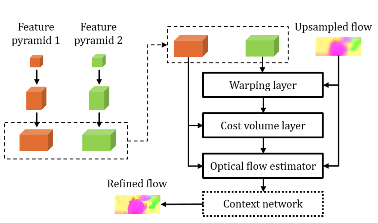
As briefly mentioned in the introduction, PWC-Net seems to have been inspired by the approach of classical coarse-to-fine optical flow algorithms. If we focus only on the PWC part of the name, we can understand the meaning of this model more easily. From now on, we will take a closer look at each component of PWC.
12.1.1. Pyramid Structure
Image pyramid is a traditional technique used in the fields of image processing and computer vision. This idea has also been adopted in ML/DL-based optical flow algorithms, and is extensively described in SpyNet [CPVR 2017]. (Since this post does not cover SpyNet, please refer to its reference for more information.)

The Pyramid Structure is a structure that obtains Optical Flow by upscaling the down-scaled input image. This helps to compensate for one of the weaknesses of Optical Flow, which is Large Motion Displacement. By securing information about Large Displacement in the Downscale process and securing detail (Small Displacement) in the Upscaling process, it shows strong resistance to large changes.
In PWC-Net, this Pyramid Structure is represented as a Learnable feature pyramid. Unlike the classical method that used raw images as input, feature maps are used as input. Two input images pass through a convolution layer and create an L-level pyramid based on the feature map by downsampling.
12.1.2. Warping Layer (Backward Warping)
Warping refers to the process of adding the up-scaled previous pyramid's flow to the second image. Optical flow obtained from an operation, not a predicted value, is used to move the actual image. In other words, the motion vector obtained by up-scaling the flow from the previous pyramid is added to $Input \,\, Image_1$. This results in the creation of Groundtruth $Input \,\, Image_2$ and $Input \,\, Image_2'$ through warping. These two may be similar, but they will not be exactly the same, and the smaller the error, the more accurate the operation is.
Why is this process important? If warping is done, learning can be done L times (L-level pyramid structure) through a single training. During the down-scaling → up-scaling process, the error between $Input \,\, Image_2$ and $Input \,\, Image_2'$ can be added as a weight in real-time. (It can be differentiated using bilinear interpolation, and end-to-end operation can be performed.)
In summary, warping improves training efficiency and allows for real-time compensation for geometric distortion by estimating errors in large motion.
12.1.3. Cost Volume Layer (Correlation Layer)
The Cost Volume (Correlation Layer) is a concept proposed in FlowNet [ICCV 2015], which stores matching costs between pixels by performing inner product operations between feature maps. Detailed concepts for this have already been covered in the FlowNet chapter, so please refer to the chapter 10 and 11. Here, in order to reduce computational costs, the Cost Volume is computed between feature maps instead of raw images.
$$\mathbf{cv}^l(\mathbf{x_1, x_2})=\frac{1}{N}(\mathbf{c}^l_1(\mathbf{x_1}))^T\mathbf{c}^l_w(\mathbf{x_2})$$
12.1.4. Optical Flow Estimator & Context Network
The Optical Flow Estimator and the Context Network both produce Optical Flow as their output. The difference is that the former outputs the Optical Flow prediction for each level of the Pyramid Structure, while the latter outputs the overall result.
- Optical Flow Estimator: Receives $Input \,\, Image_1$, Cost Volume, and Upsampled Flow as inputs to predict Optical Flow for each level of the Pyramid.
- Context Network: Combines the Optical Flow generated at each level of the multi-level pyramid into one (Refined Flow).
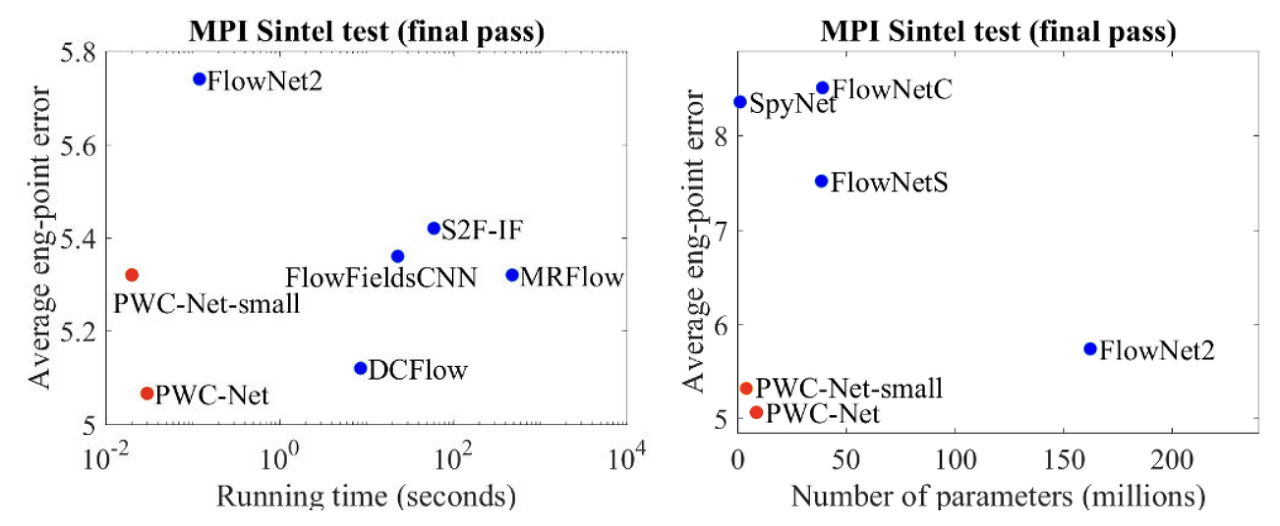
12.2. Result

13. RAFT (ECCV 2020)
In this chapter, we will talk about RAFT: Recurrent All-Pairs Field Transforms for Optical Flow. The most impressive part of this paper was the Optical Flow iteration, which will be explained in detail later. In simple terms, it is a process of iteratively improving the accuracy of the result through repetitive computation. The reason why this was impressive is that I had added only the idea of this process while writing my graduation thesis, but I eventually failed to carry it out. However, since the related content is described in the paper, I will briefly discuss it in appendix after introducing RAFT.
RAFT is a paper that achieved remarkable performance. Usually, the Best Paper award would go to papers that propose groundbreaking techniques or approaches that become game changers. However, RAFT focused on performance and technical aspects rather than novelty. Nevertheless, the overwhelming impression given by its exceptional performance was likely a significant factor in winning the Best Paper Award.
However, if you ask whether there is no entirely new algorithm, the answer would be no. Previously, Optical Flow calculations typically concatenated the results after changing Scale/Sampling, and then obtained the final answer. RAFT proposed a recursive iterative approach to move towards the final answer, without using ground truth/labeling, which I believe is a reasonable method in fields where evaluation is possible to some extent.
As mentioned earlier, this part is relevant to my research field. While working on a task using FlowNet2.0, I once thought that it would be great to move towards the correct answer by iterating like the Gradient Descent algorithm. I was inspired by the algorithm that was being developed using reinforcement learning in the lab. However, the overhead caused by repeated correlation volume calculations could not be overcome, and it was eventually excluded from the final task results.
It would be helpful to look at how RAFT was able to drastically reduce the correlation calculation in the upcoming content as another important point.
13.1. Energy Minimization
RAFT borrows some parts from classical Optical Flow algorithms. It optimizes by minimizing the Optical Flow Constraint and incorporates iterations into this process, which is where the idea comes from. We have already introduced the Optical Flow Constraint in a previous chapter, so please refer to the chapter 4 for more information on this topic.
13.2. Architecture
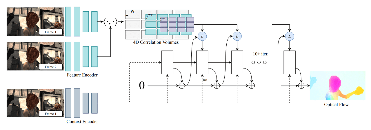
RAFT can be divided into three main parts: Feature Encoder, Context Encoder for feature extraction, Correlation Layer for creating the Correlation Volume between images, and Update Operator for updating and refining the Flow Field from an initial value [Zero] through iterations. Through this three-stage architecture, RAFT computes Optical Flow in the following order:
- Feature Extraction
- Computing Visual Similarity
- Iterative Updates
13.2.1. Feature Extraction
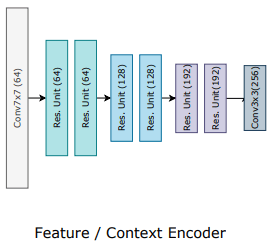
Feature extraction plays a critical role in optical flow estimation, as it is responsible for computing visual similarity between two input frames. RAFT employs a feature extractor composed of two sub-networks: Feature Encoder Network (F-Net) and Context Encoder Network (C-Net).
F-Net is a convolutional neural network (CNN) that extracts features from down-sampled images. It computes a feature vector for each pixel of the input frames, generating feature maps for Frame 1 and Frame 2. The feature maps are then used to compute the visual similarity between the two frames, which is a critical step in the optical flow estimation process.
On the other hand, C-Net extracts context features from Frame 1. It is similar in structure to F-Net, but it only extracts features from Frame 1 to capture its contextual information. This feature map is fed to the Update Operator as an input to refine and update the flow field iteratively.
Both F-Net and C-Net are based on a ResNet architecture and produce 256-channel feature maps. By extracting feature maps from both frames and capturing the contextual information, RAFT is able to compute optical flow accurately and robustly.
13.2.2. 4D Correlation Layer (Correlation Volume)

The correlation layer, which has been used in optical flow models since FlowNet, is also used in RAFT. Since we have already covered the basic concepts of the correlation layer in the review of FlowNet/FlowNet2.0, we will not cover it in detail here. However, the figure 38 does an excellent job of explaining what it means to create a correlation volume, so I decided to include it. Before delving into the correlation layer of RAFT, if you want to learn more about the correlation layer used in optical flow models in general, please refer the chapter 10 and 11.
In RAFT, there is a slight difference between the timing of generating and using the correlation volume. This can be divided into before and after the iteration process based on the entry point of the Update operator. Let's take a closer look at this aspect.
13.2.2.1. 4D Correlation Volume Generation - Before Iteration
$$\mathbf{C}(g_\theta (I_1),g_\theta (I_2))\in \mathbb{R}^{H\times W \times H \times W}, \quad\quad C_{ijkl}=\sum_{h}g_\theta (I_1)_{ijh}\cdot g_\theta (I_2)_{klh} $$
Unlike conventional correlation, RAFT generates a 4D correlation volume. As shown in the equation above, it stores the results of $Image_{1}(i, j)\cdot Image_{2}(k, l)$. As a result of the equation, a tensor of $H_{1} \times W_{1}$ is created, each with a size of $H_{2} \times W_{2}$. That is, the total size is $H_{1} \times W_{1} \times H_{2} \times W_{2}$.
$$C^k:\begin{bmatrix}H \times W \times \frac{H}{2^k} \times \frac{W}{2^k}
\end{bmatrix}$$
One special point can be seen in figure 38. With the above equation, we can obtain the result for $C^{1}$. From now on, we generate the Correlation Pyramid by downsampling, using average pooling with kernel sizes of {1, 2, 4, 8}, resulting in $C^{1}, C^{2}, C^{3}, C^{4}$ as the final outputs. The use of average pooling is a good approach to quickly compute coarse correlation.
We now have a deterministic Correlation Pyramid for $Image_{1}$ and $Image_{2}$. Therefore, during the iteration process, we can significantly reduce the overhead by not performing correlation calculations separately.
13.2.2.2. Correlation Lookup - During Iteration
After entering the Update operator, the precomputed Correlation volume is referenced through the Correlation Lookup process. The Correlation volume is bilinearly sampled around the location corresponding to the current Optical Flow. The 3D Correlation feature is obtained by using the sampled Correlation volume and the Current Optical Flow. Finally, the resulting $(2r+1)^2$ vectors for each Target point are reshaped into a tensor of size $H \times W \times (2r+1)^2$.
13.2.3. Update Operator
RAFT uses a GRU structure to gradually approach a more accurate flow field as it iterates. This can be thought of as stacking layers recursively using CNNs, which has a very similar shape to RNNs (in fact, it is same). Understanding RNN-like architectures has become increasingly important in the computer vision field as transformers continue to invade. However, in this chapter, we will simply summarize and move on.
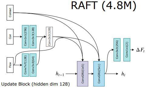
In figure 39, three inputs are combined and fed into the ConvGRU, which is the Update operator. The previous hidden state is also added to these inputs to form the final input, and the output is passed through an additional convolutional layer. This process determines the current Flow field, which can be iteratively updated to obtain the final Flow field.
- Inputs
- $x_{t}$: Encoded previous Optical Flow + Encoded Correlation lookup + Output of C-Net
- $h_{t-1}$: Previous hidden state, which is a hidden unit of GRU.
During the iteration process, the Flow field is updated according to the following equation:
$$f_{k+1}=f_{k}+ \bigtriangleup{f_{k}}$$
Here, $\bigtriangleup{f_{k}}$ is the Flow field that results from the iteration, and the output is updated from an initial value of 0. This is reasonable since there is no previous frame or any change in the initial state. The paper extensively discusses the iteration process and its considerations. We will explore these points in next chapter.
13.3. Iteration
In RAFT, there are two main aspects to consider with respect to iterations: training and inference. Let's take a look at each one.
13.3.1. Training
The training process of RAFT follows a form where the loss becomes more significant as the iteration progresses. Although a straightforward and reliable method is chosen to calculate the error loss with the ground truth, it reflects the features well by comparing all feature maps in the iteration with the ground truth. In this case, if the iteration increases, the weight also increases. The experimental optimal value is shown as $\gamma=0.8$ in the equation below.
$$L=\sum_{i=1}^{N}\gamma ^{i-N}\left\|\mathbf{f}_{gt}-\mathbf{f}_i \right\|_1$$
13.3.2. Inference
In inference, there are two methods called Zero Initialization and Warm Start that consider iteration. Zero Initialization sets the initial value of the Flow field to 0, and since it has already been examined, it will not be further discussed. Warm Start is a method proposed to utilize the previous flow, and it is a Forward Projection technique that actually moves and uses it for the next initialization. This is to utilize the previous flow field as a guide in the next iteration, and the following equation is used for this purpose:
$$f_{t}(x+f_{t-1}(x))=f_{t-1}(x)$$
13.4. Result
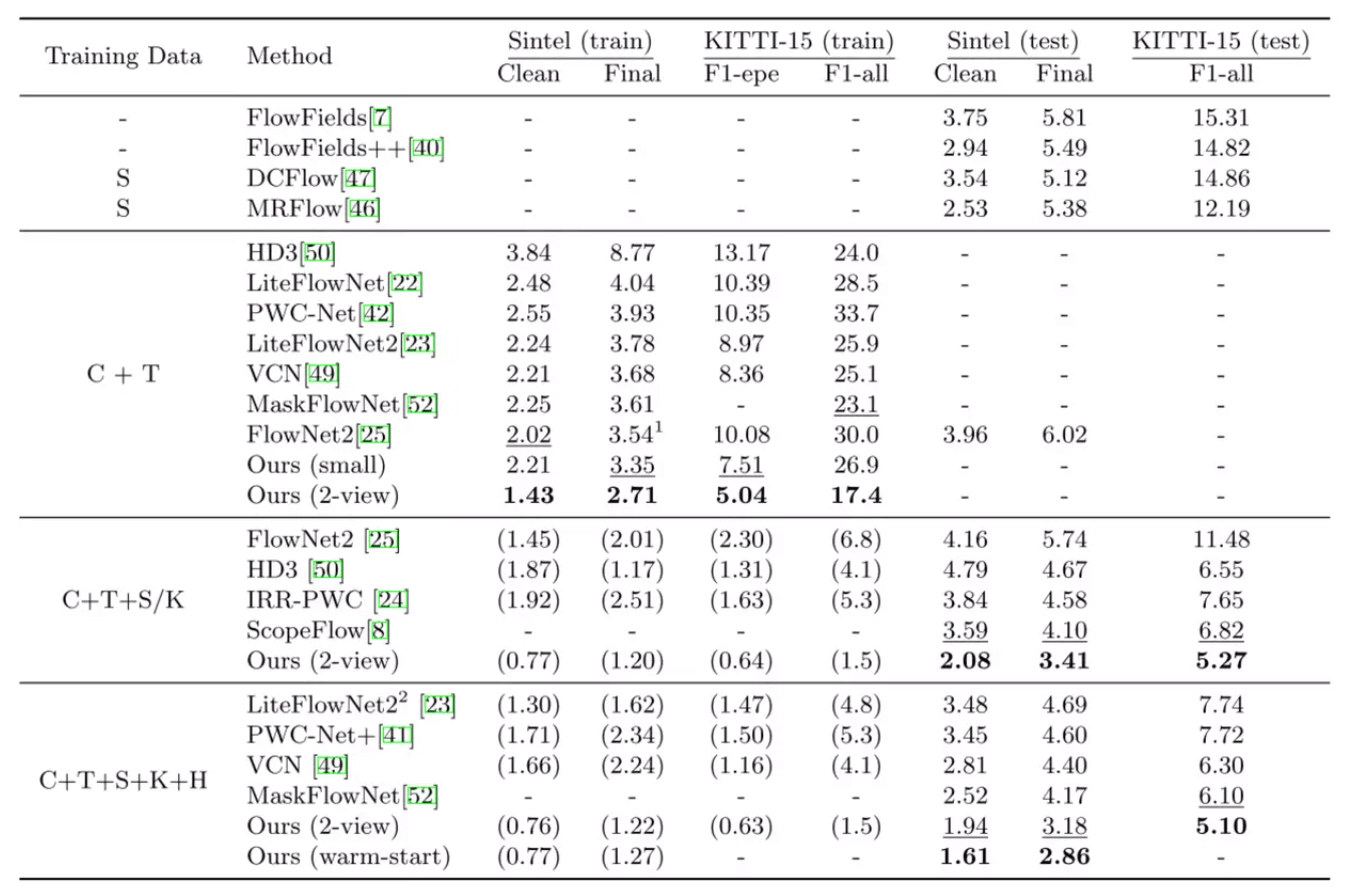
13.4.1. EPE [End-Point-Error]
13.4.2. Performance Plot

14. Reference
- Lucas-Kanade Algorithm
Scale Space와 이미지 피라미드(image pyramid)
문일지십. 하나를 들으면 열을 깨닫는다. 보통은 머리가 뛰어난 사람을 일컫는 말이지만 꼭 그런 것만은 아니라고 생각한다. 우리가 어떤 잘 모르는 개념 또는 사물을 알고 싶을 때 한눈에 깨닫
darkpgmr.tistory.com
[optical flow] Lucas-Kanade method with pyramid
개념정리문제 optical flow를 적용하기 위한 가장 중요한 가정(전제)은? optical flow equation과 각 항들이 의미하는바는? Lucas-Kanade 기법을 쓰는 이유 Lucas-Kanade의 단점을 보완하기 위한 방법은? 위 질문
powerofsummary.tistory.com
- EpicFlow
EpicFlow: Edge-Preserving Interpolation of Correspondences for Optical Flow
We propose a novel approach for optical flow estimation , targeted at large displacements with significant oc-clusions. It consists of two steps: i) dense matching by edge-preserving interpolation from a sparse set of matches; ii) variational energy minimi
arxiv.org
[컴퓨터비젼] 6. Feature descriptors and matching
오늘은 Feature descriptor 와 matching 에 대해서 알아보도록 합시다. 저번 포스팅에서도 언급을 했듯이 Feature을 찾는 과정은 Detection, Description, Matching 으로 이루어져있습니다. 일단 Feature descriptor의 정
com24everyday.tistory.com
- FlowNet/FlowNet2.0
FlowNet: Learning Optical Flow with Convolutional Networks
Convolutional neural networks (CNNs) have recently been very successful in a variety of computer vision tasks, especially on those linked to recognition. Optical flow estimation has not been among the tasks where CNNs were successful. In this paper we cons
arxiv.org
FlowNet 2.0: Evolution of Optical Flow Estimation with Deep Networks
The FlowNet demonstrated that optical flow estimation can be cast as a learning problem. However, the state of the art with regard to the quality of the flow has still been defined by traditional methods. Particularly on small displacements and real-world
arxiv.org
PR-214: FlowNet: Learning Optical Flow with Convolutional Networks
제 PR12 첫번째 발표 논문은 FlowNet이라는 논문입니다. Optical Flow는 비디오의 인접한 Frame에 대하여 각 Pixel이 첫 번째 Frame에서 두 번째 Frame으로 얼마나 이동했는지의 Vector를 모든 위치에 대하여 나
www.slideshare.net
- PWC-Net
PWC-Net: CNNs for Optical Flow Using Pyramid, Warping, and Cost Volume
We present a compact but effective CNN model for optical flow, called PWC-Net. PWC-Net has been designed according to simple and well-established principles: pyramidal processing, warping, and the use of a cost volume. Cast in a learnable feature pyramid,
arxiv.org
Optical Flow Estimation using a Spatial Pyramid Network
We learn to compute optical flow by combining a classical spatial-pyramid formulation with deep learning. This estimates large motions in a coarse-to-fine approach by warping one image of a pair at each pyramid level by the current flow estimate and comput
arxiv.org
[논문 읽기] PWC-Net(2017), CNNs for Optical Flow Using Pyramid, Warping, and Cost Volume
PWC-Net, CNNs for Optical Flow Using Pyramid, Warping, and Cost Volume PDF, Optical Flow, Deqing Sun, Xiaodong Yang, Ming-Yu Liu, Jan Kautz, arXiv 2017 GIST 컴퓨터 비전 과제로 제출한 결과물 입니다. Summary 해당 논문은 Optical Flow를
deep-learning-study.tistory.com
- RAFT
RAFT: Recurrent All-Pairs Field Transforms for Optical Flow
We introduce Recurrent All-Pairs Field Transforms (RAFT), a new deep network architecture for optical flow. RAFT extracts per-pixel features, builds multi-scale 4D correlation volumes for all pairs of pixels, and iteratively updates a flow field through a
arxiv.org
15. Appendix
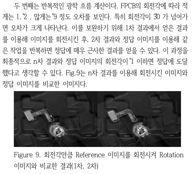
I was quite pleased with RAFT because it incorporates the method I tried in my graduation thesis. This method was able to reduce the accuracy by around 1%, but it took a long time and had the problem that it was impossible to define the processing time. In particular, the process of creating a correlation volume each time had a large overhead, and I was greatly impressed by the author of RAFT solving this problem. The content is included in section 2.6 Error Correction of the paper, and the image below captures the content.
[논문]영상을 적용한 인공지능을 이용한 Robot Arm Placing 기술 개발
최근 딥 러닝을 이용해 기계로 인간을 대체하는 스마트 팩토리에 대한 연구 및 개발이 활발히 진행되고 있다. 그러나 FPCB를 Placing하는 방법에 기계를 도입하는 과정은 발전이 더딘 상태이다. 현
scienceon.kisti.re.kr
